Session8-Tableau_07Feb

Tableau with GSS Survey Data 

Measures and Dimensions:
Sex is included under measures when it should really be a category.
That's because our data file used "1" and "2" to represent male and women, so Tableau thought it was a numerical field. Let's fix that. Simply drag SEX from the measures area and drop it in the dimensions area.

Editing Aliases and Data Labels:
Now, right click SEX, choose "Edit Mark Properties >> Aliases", change the value "1" to "Men" and the value "2" to "Women". Then right click SEX again, select "Rename" and change SEX to GENDER. That will make things less confusing when we're talking about premarital sex and frequency of sex.

Year is also included as a measure, but it should really be a category as well. We typically segment data by year, we don't add or average years together. Drag YEAR to the category box, too.

Creating Calculated Fields:
Right click SEXFREQ and choose "Describe". If you click "Load", you'll see a list of all the existing values in this field. The field contains each interviewee's response to the question "How many times did you have sex last year?" Their responses are grouped into 7 bins (plus a null value for those interviewees who gave no response or weren't asked), but it would be more interesting if we had a numerical value for each person's yearly sexual frequency.

Fortunately, we can approximate that.  Close the description dialog box, then right click in the measures area and choose "Create calculated field". Name it "SexPerYear" and paste the following code into the formula box:

Case [SEXFREQ]
When "Not at all" Then 0
When "Once or twice" Then 1.5
When "Once a month" Then 12
When "2-3 times a month" Then 30
When "Weekly" Then 52
When "2-3 times per week" Then 130
When "4+ times per week" Then 250
Else Null
End

Drag and Drop Data Visualization:
Drag YEAR to the columns shelf and drag SexPerYear to the rows shelf. The default aggregation is sum, so we're looking at the total number of times all survey respondents had sex each year. Since there were different numbers of people surveyed each year, this chart isn't particularly informative. Right click SUM(SexPerYear) on the Rows shelf and select "Measure (SUM) >> Average". Now we have the average number of times survey respondents had sex every year.

Answering Questions with Visual Analysis:
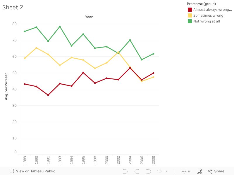
Now we start to ask questions. What effect do you think an interviewee's opinion on premarital sex has on the number of times they have sex each year? Drag PREMARSX to the color shelf to find out.

I'm curious about trends over time, so change marks to Line. The line for NULL (people who weren't asked this survey question) doesn't tell us anything, so right click NULL in the color legend and choose "Exclude".

Grouping Data Set Members:
Let's say we've also decided that we don't really need to differentiate between people who think premarital sex is "always wrong" and those who think it's "almost always wrong". Instead, we'll group them together. By holding down the control key, select "almost always wrong" and "always wrong", right click, and choose "group".

We have an interesting result already. Over the past 20 years, those opposed to premarital sex have been having more and more sex on average each year, while those who think it is not wrong at all have been having less and less. Why do you think this is?

Editing Marks and Color Legends:
We're going to attempt to answer this question, but to make our graph even easier to understand, let's change the color legend. Right click inside the color legend and select "Edit Colors".  Change the Color Palette dropdown from Automatic to Traffic Light. Click on the "Almost always wrong, Always wrong" group and then select a nice shade of red. Click "Not wrong at all" and select a shade of green, and then select "Sometimes wrong" and select a shade of yellow. Close and then in the color legend, drag "Not wrong at all" to the bottom so the opinions are in order.

We don't want to confuse correlation with causality, though. It's probable that there's a confounding variable at work here, and one of the most likely culprits is age. Let's look at how the average age of these three groups has changed over the years.

Editing an Existing Visualization:
Right click on the "Sheet 1" tab at the bottom of the Tableau window and choose "Duplicate sheet". On the new sheet, "Sheet 2", drag Age from the Measures box and drop it directly on top of the "AVG(SexPerYear)" field on the Rows shelf. "AVG(SexPerYear)" will disappear and be replaced with "SUM(AGE)". Right click "SUM(AGE)" and select  "Measure (SUM) >> Average". We see now that the average age of those opposing premarital sex has been decreasing, while the average age of those supporting it has been increasing.

The question remains, however, why is the demographic makeup of these groups changing? Why would the average premarital sex opponent be getting younger and younger? Does it have something to do with recent trends in abstinence education? That seems unlikely, as the shift in age has been going on for twenty years.

Let's examine more closely the changing opinions among the young and the old. Create a new calculated field, this time in the dimensions box. For name, put "Binned Age (<40)" and paste the following into the formula:

IF [AGE]<40 THEN '<40'

ELSE '40+'

END

Switching Between Different Chart Types:
Duplicate Sheet 2, and on the new sheet, switch the Marks dropdown menu from "Line" to "Bar". Drag "Number of Records" from the Measures box to the rows shelf and use it to replace the "AVG(AGE)" field. We can now see how many respondents each year had each opinion on premarital sex. However, the total number of respondents each year vary by quite a bit, so looking at percentages will make the graph much more understandable.

Calculating Percentages:
From the Analysis menu, choose "Percentage of >> Cell". It appears that acceptance of premarital sex is slowly growing among the general population. However, we were particularly interested in how opinions were changing within age brackets. So drag the "Binned Age (<40)" dimension to the column shelf and drop it to the left of YEAR. The answer appears when we segment the population into under-40 and over-40 age brackets. In the under-40 age bracket, beliefs have remained remarkably consistent over the past twenty years. In the over-40 age bracket, on the other hand, there has been a clear shift towards increased acceptance of premarital sex.

Session7-Tableau_03Feb

My first Tableau sheet

Session6-Plotting graphs with seaborn_31Jan

Different cubehelix palettes:

!pip install seaborn

import numpy as np
import seaborn as sns
import matplotlib.pyplot as plt

%matplotlib inline
sns.set(style="dark")
rs = np.random.RandomState(50)

# Set up the matplotlib figure
f, axes = plt.subplots(3, 3, figsize=(9, 9), sharex=True, sharey=True)
# Rotate the starting point around the cubehelix hue circle
for ax, s in zip(axes.flat, np.linspace(0, 3, 10)):

    # Create a cubehelix colormap to use with kdeplot
    cmap = sns.cubehelix_palette(start=s, light=1, as_cmap=True)

    # Generate and plot a random bivariate dataset
    x, y = rs.randn(2, 50)
    sns.kdeplot(x, y, cmap=cmap, shade=True, cut=5, ax=ax)
    ax.set(xlim=(-3, 3), ylim=(-3, 3))

f.tight_layout()

Discovering structure in heatmap data:

!pip install seaborn

import pandas as pd
import seaborn as sns
import matplotlib.pyplot as plt
sns.set(font="monospace")

%matplotlib inline
# Load the brain networks example dataset
df = sns.load_dataset("brain_networks", header=[0, 1, 2], index_col=0)

# Select a subset of the networks
used_networks = [1, 5, 6, 7, 8, 11, 12, 13, 16, 17]
used_columns = (df.columns.get_level_values("network")
                          .astype(int)
                          .isin(used_networks))
df = df.loc[:, used_columns]

# Create a custom palette to identify the networks
network_pal = sns.cubehelix_palette(len(used_networks),
                                    light=.9, dark=.1, reverse=True,
                                    start=1, rot=-2)
network_lut = dict(zip(map(str, used_networks), network_pal))

# Convert the palette to vectors that will be drawn on the side of the matrix
networks = df.columns.get_level_values("network")
network_colors = pd.Series(networks, index=df.columns).map(network_lut)

# Create a custom colormap for the heatmap values
cmap = sns.diverging_palette(h_neg=210, h_pos=350, s=90, l=30, as_cmap=True)

# Draw the full plot
sns.clustermap(df.corr(), row_colors=network_colors, linewidths=.5,
               col_colors=network_colors, figsize=(13, 13), cmap=cmap)

Multiple linear regression:

import seaborn as sns
sns.set(style="ticks", context="talk")

# Load the example tips dataset
tips = sns.load_dataset("tips")

# Make a custom sequential palette using the cubehelix system
pal = sns.cubehelix_palette(4, 1.5, .75, light=.6, dark=.2)

# Plot tip as a function of toal bill across days
g = sns.lmplot(x="total_bill", y="tip", hue="day", data=tips,
               palette=pal, size=7)

# Use more informative axis labels than are provided by default
g.set_axis_labels("Total bill ($)", "Tip ($)")

Scatterplot Matrix:

import seaborn as sns
sns.set()

df = sns.load_dataset("iris")
sns.pairplot(df, hue="species")

Scatterplot with categorical variables:

import pandas as pd
import seaborn as sns
sns.set(style="whitegrid", palette="muted")

# Load the example iris dataset
iris = sns.load_dataset("iris")

# "Melt" the dataset to "long-form" or "tidy" representation
iris = pd.melt(iris, "species", var_name="measurement")

# Draw a categorical scatterplot to show each observation
sns.swarmplot(x="measurement", y="value", hue="species", data=iris)

Grouped Boxplots:

import seaborn as sns
sns.set(style="ticks")

# Load the example tips dataset
tips = sns.load_dataset("tips")

# Draw a nested boxplot to show bills by day and sex
sns.boxplot(x="day", y="total_bill", hue="sex", data=tips, palette="PRGn")
sns.despine(offset=10, trim=True)

Session5-Plotting Cities on Map with data_25Jan

Here we have data about number of registered vehicles in different years in this spreadsheet - Google Docs spreadsheet. And, we use this data to draw the Google GeoChart.

We need to do a little tweaking to the html code, which executes our map display function.

We need to get GoogleMaps API Credentials - meaning, we get an API Key from the below link:
https://developers.google.com/maps/documentation/javascript/get-api-key

And, add this to the second line of code of the executable map display html code.

Session4-Web hosting with charts_16Jan

Scatterplot Matrix

Document content goes here...

The scatterplot matrix visualizations pairwise correlations for multi-dimensional data; each cell in the matrix is a scatterplot.

Session3-My First Google Charts-part4_12Jan

Creating a Dashboard - Part II

Here we take the same data used in the previous post and convert it into a dashboard. We have replaced the chart with a chart wrapper. Added three filters. Added a dashboard component and bound the three filters to the chart wrapper. You can see the result both in this blog as well as on this regular HTML page.

The Dashboard on this blog

Data Source

One can choose one or multiple states. Also one can specify the range of cow and buffalo milk production and so select only the states that have this production.

Session3-My First Google Charts-part3_12Jan

Creating a Dashboard - Part 1

When you have a lot of data to be shown on a page, it makes sense to give the viewer an opportunity to filter some of the data so that he or she gets a cleaner view. In this case, we will first draw a rather clumsy Column Chart and then in the next section. The data for the chart is drawn from this spreadsheet. The chart shown below can also be seen in this regular HTML page.

Basic Column Chart Showing All Data

Data Source


Linkfor Data Source

Note how we have specified:

• the Google Docs spreadsheet : https://docs.google.com/spreadsheets/d/1k0xYnDU78GYGuMivC-JTD3AakxyftIS4-Z_ptboPsQs/edit?usp=sharing
• the sheet : sheet=MilkProduction
• range : range=B2:H37
• headers : headers=1
• columns : query.setQuery('select B,E,F');
• chart type : var chartMQ = new google.visualization.ColumnChart(document.getElementById('chart_divMQ'));